How to Calculate a 95% Confidence Interval: Worked Example

To calculate a 95% confidence interval for a population mean, take the sample mean and add and subtract a margin of error. When the population standard deviation is unknown, the margin of error is the appropriate t critical value multiplied by the sample standard deviation divided by the square root of the sample size. In short: estimate ± critical value × standard error.

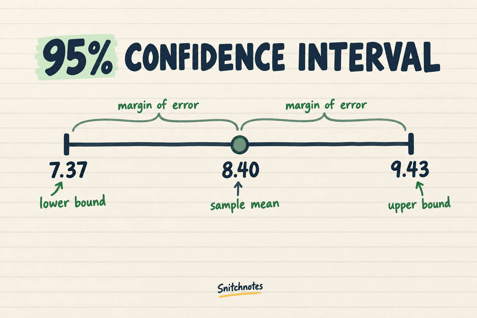
We will calculate one from start to finish using 25 café wait times. The sample mean is 8.40 minutes and the sample standard deviation is 2.50 minutes. The final 95% confidence interval is 7.37 to 9.43 minutes. The arithmetic is short; choosing the right formula and interpreting the result are where the real learning happens.

The formula and what each part means

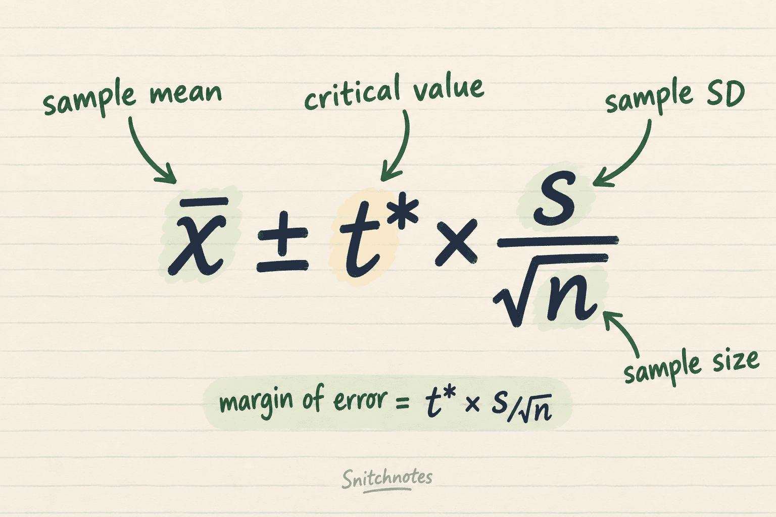
For a one-sample confidence interval for a mean when the population standard deviation is unknown, use x̄ ± t* × s/√n. Here x̄ is the sample mean, s is the sample standard deviation, n is the sample size, and t* is the critical value from Student's t distribution. The quantity s/√n is the standard error of the sample mean.

The standard error describes how much sample means would typically vary from sample to sample. Multiplying it by the critical value creates the margin of error. Subtract that margin from the sample mean for the lower bound, then add it for the upper bound.

Worked example: café wait times

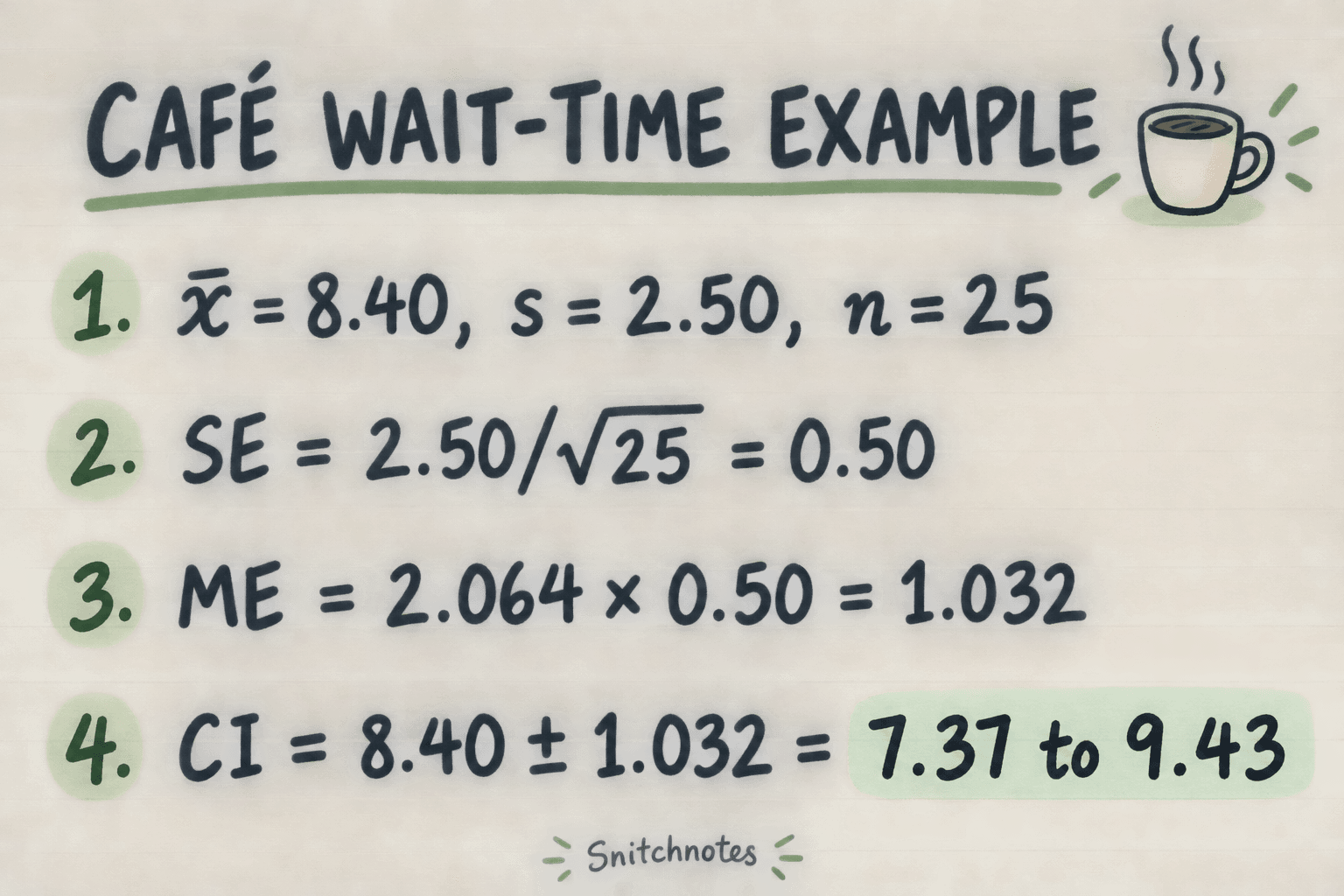
Maya manages a campus café and wants to estimate the average lunchtime wait for all customers. She records a reasonably representative sample of 25 waits. The sample has a mean of 8.40 minutes and a standard deviation of 2.50 minutes. Because the population standard deviation is unknown, she uses a t interval rather than simply inserting the normal critical value 1.96.

Step 1: Calculate the standard error

Divide the sample standard deviation by the square root of the sample size: SE = 2.50/√25 = 2.50/5 = 0.50 minute. The standard error is smaller than the spread of individual wait times because it measures uncertainty in the mean, not variation among individual customers.

Step 2: Find the 95% critical value

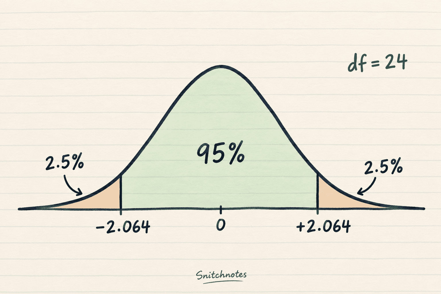
A one-sample t interval has n − 1 degrees of freedom, so this example has 25 − 1 = 24. For a two-sided 95% interval with 24 degrees of freedom, the critical value is about 2.064. The central 95% sits between −2.064 and +2.064, leaving 2.5% in each tail. You can obtain this value from a t table, calculator, or statistics software.

Step 3: Find the margin of error

Multiply the critical value by the standard error: ME = 2.064 × 0.50 = 1.032 minutes. This is the distance from the sample mean to either end of the interval. Rounding too early can shift the endpoints, so keep a few extra decimal places until the final line.

Step 4: Calculate the lower and upper bounds

Lower bound: 8.40 − 1.032 = 7.368. Upper bound: 8.40 + 1.032 = 9.432. Rounded to two decimal places, the 95% confidence interval is 7.37 to 9.43 minutes. A compact report would be: mean wait = 8.40 minutes, 95% CI [7.37, 9.43].

How to interpret a 95% confidence interval

In context, Maya can say she is 95% confident that the population mean lunchtime wait is between 7.37 and 9.43 minutes, provided the sampling method and model assumptions are reasonable. The interval estimates the mean wait for the population represented by her sample. It does not say that 95% of individual customers wait inside that range.

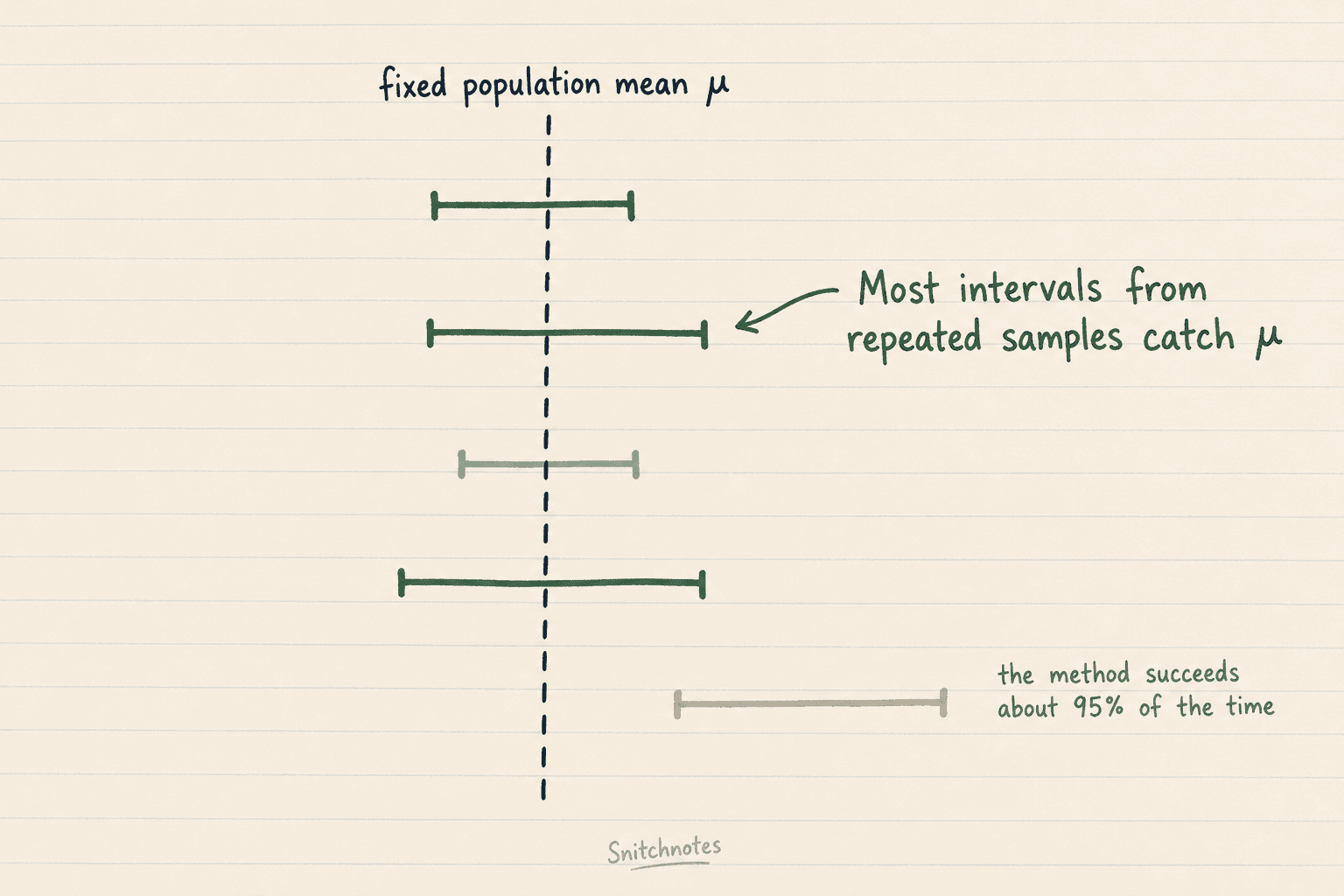
The careful frequentist interpretation concerns the method: if Maya repeatedly drew samples in the same way and built an interval each time, about 95% of those intervals would contain the fixed population mean. After this particular interval is calculated, the endpoints are fixed. Saying there is a 95% probability that the fixed mean lies inside this specific interval is a common but technically incorrect shortcut.

When this calculation is appropriate

A one-sample t interval is designed for quantitative observations that are independent and collected through a defensible random or representative process. For a small sample, the population distribution should be roughly normal and free of severe skew or influential outliers. With larger samples, the sampling distribution of the mean is often approximately normal under broad conditions, but bad sampling cannot be repaired by a larger n.

Use a different procedure for paired before-and-after data, two independent groups, proportions, or strongly dependent observations. If the population standard deviation is genuinely known, a z interval uses the normal critical value 1.96 for 95% confidence. In most classroom and real-world mean problems, however, the population standard deviation is unknown, so the t interval is the usual choice.

What changes the width of the interval?

More uncertainty produces a wider interval. A larger sample standard deviation increases the standard error. A higher confidence level uses a larger critical value. A larger sample size usually narrows the interval because n appears under a square root: quadrupling n cuts the standard error in half when the sample standard deviation stays similar. Narrower is not automatically better if the data are biased or poorly collected.

Check your understanding

Suppose Maya kept the same mean and standard deviation but collected 100 independent waits. What happens to the standard error? It becomes 2.50/√100 = 0.25 minute, half the original 0.50. The interval would therefore be narrower, although the exact margin would use the t critical value for 99 degrees of freedom.

Now spot the misconception: “95% of customers wait between 7.37 and 9.43 minutes.” That is wrong because the interval concerns the population mean, not the distribution of individual waits. Individual wait times can vary much more widely than the estimated mean.

Related concepts

Statistical significance versus practical importance helps you decide whether a statistically detectable result is large enough to matter. How to study statistics word problems offers a repeatable way to translate a prompt into the right statistical procedure.

When formulas start blurring together, Snitchnotes can turn your lecture notes or PDFs into clearer study notes, quizzes, and flashcards for practice.

Sources

National Institute of Standards and Technology: Confidence Limits for the Mean

National Institute of Standards and Technology: Critical Values of the Student's t Distribution

Penn State STAT 415: A t-Interval for a Mean

OpenStax Introductory Statistics 2e: A Single Population Mean Using the Student t Distribution