
Snitchnotes Team
How to Study Eigenvalues and Eigenvectors With Transformation Sketches
How to Study Eigenvalues and Eigenvectors With Transformation Sketches
To understand eigenvalues and eigenvectors, stop treating Av = λv as a formula to memorize and read it as a transformation sketch. A matrix A moves vectors. An eigenvector v is a nonzero vector whose image Av stays on the same line through the origin; the eigenvalue λ tells you how much that vector is stretched, squeezed, reversed, or collapsed.
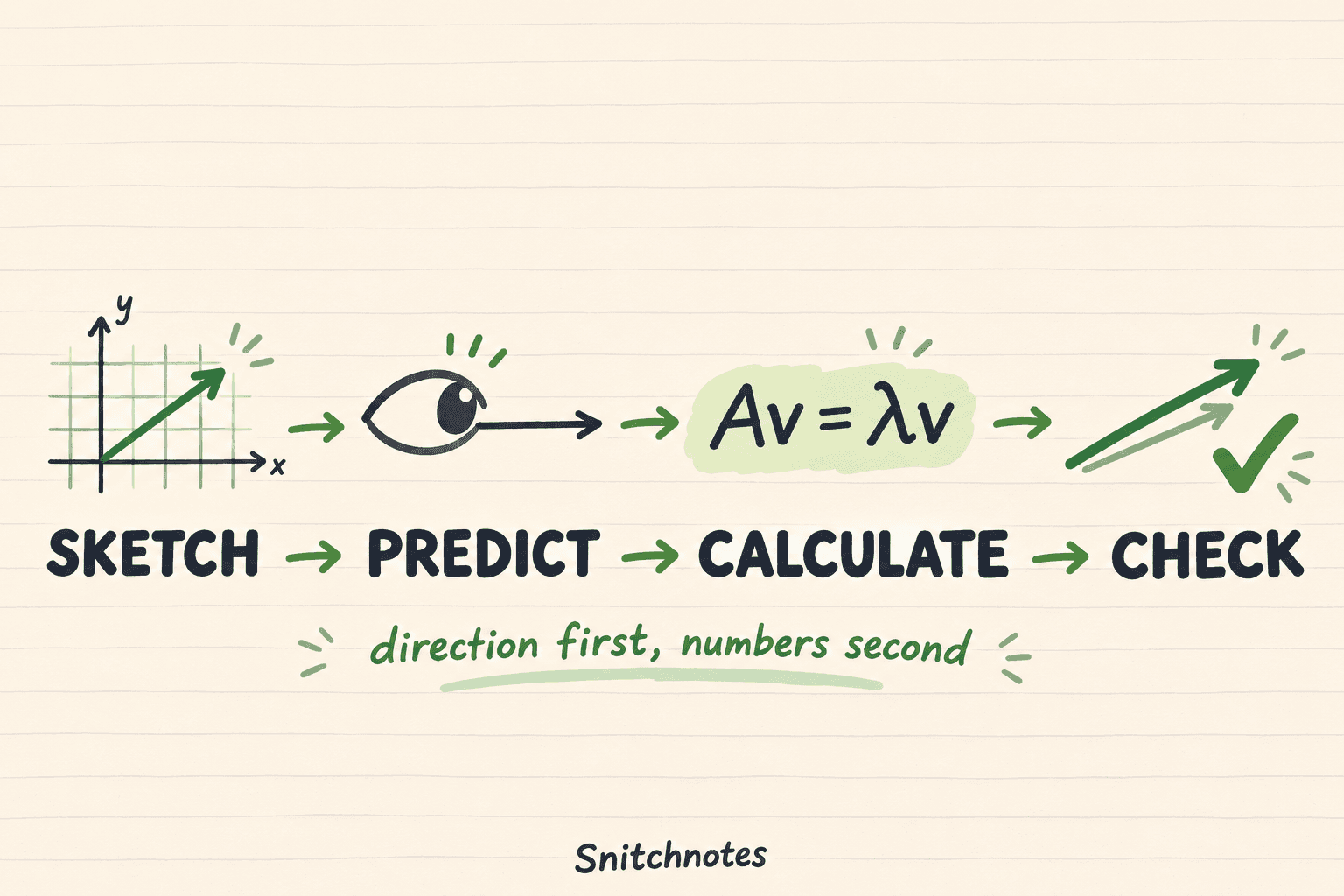
This article is for students who can perform matrix multiplication but still find the idea mysterious. The most useful study order is sketch, predict, calculate, check. Geometry gives the symbols a job, and the algebra confirms whether your picture is right.
What eigenvalues and eigenvectors mean
A square matrix represents a linear transformation. Most vectors change both length and direction when the transformation acts. Eigenvectors are the special nonzero vectors that do not get pushed off their original line. In Av = λv, the left side applies the transformation, while the right side says the result is only a scalar multiple of the starting vector.
The value of λ describes what happens along that eigenvector direction. If λ is greater than 1, the vector grows. If 0 < λ < 1, it shrinks. A negative λ reverses its direction as well as scaling it, and λ = 0 sends it to the zero vector. The transformed arrow may point backward, but it still lies on the same line.
Georgia Tech's Interactive Linear Algebra expresses the geometry precisely: v and Av are collinear with the origin. That wording is better than saying an eigenvector “does not move.” It can change dramatically in length or orientation; what it preserves is its one-dimensional span.
Why the transformation sketch matters
The determinant method can produce correct numbers without explaining them. A sketch makes you ask the conceptual question first: which directions does this transformation leave on their own lines? For a horizontal stretch and vertical squeeze, the coordinate axes are natural candidates. For a reflection, the mirror line and the perpendicular direction are candidates.
The sketch is not a substitute for proof. It is a prediction tool and an error detector. If your algebra claims that a diagonal stretch sends (1, 0) to a tilted vector, the picture tells you immediately that a multiplication or transcription error has occurred.
Use the sketch-predict-calculate-check routine
- Sketch: draw a few simple vectors or a unit square and show what A does to them. Focus on direction before exact scale.
- Predict: mark any nonzero directions that appear to remain on the same line through the origin. Predict whether each grows, shrinks, reverses, or collapses.
- Calculate: solve det(A − λI) = 0 for the eigenvalues. For each λ, solve (A − λI)v = 0 for nonzero eigenvectors.
- Check: multiply A by each candidate v and verify that the result equals λv exactly. Then compare the result with your sketch.
Repeat the routine from a blank page rather than rereading a completed solution. Your goal is to retrieve the meaning of each step: preserved line, scale factor, characteristic equation, and direct verification.
Worked example: stretch x and squeeze y
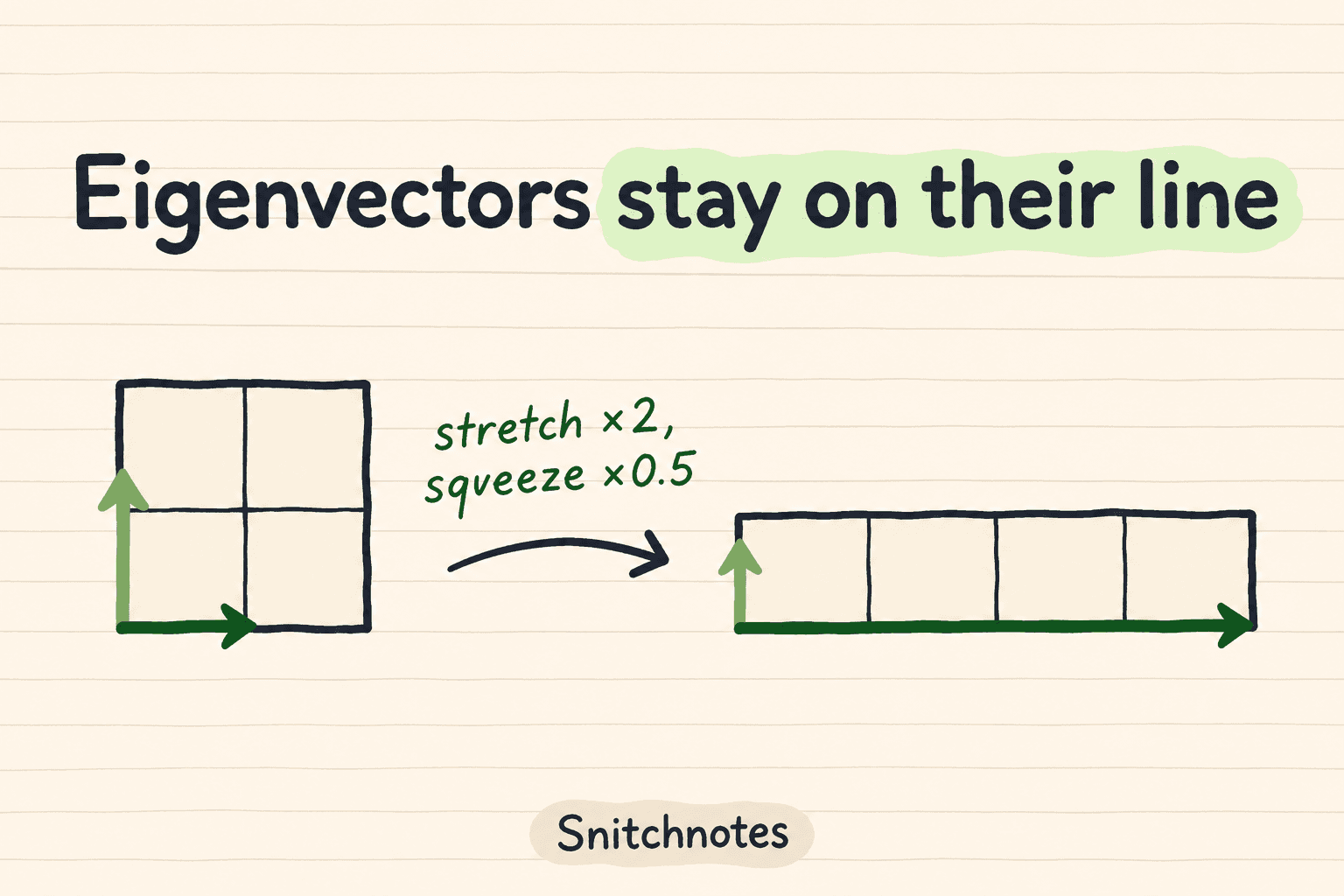
Let A = [[2, 0], [0, 0.5]]. Sketch a unit square. The matrix doubles every x-coordinate and halves every y-coordinate, so the square becomes a rectangle that is twice as wide and half as tall. Before calculating, predict that the x-axis and y-axis directions will remain aligned.
Now calculate. The characteristic equation is det(A − λI) = (2 − λ)(0.5 − λ) = 0, so the eigenvalues are 2 and 0.5. For λ = 2, solving (A − 2I)v = 0 gives vectors of the form (x, 0), with x ≠ 0. For λ = 0.5, the solutions have the form (0, y), with y ≠ 0.
Finally, check one representative from each direction. A(1, 0) = (2, 0) = 2(1, 0), so (1, 0) is an eigenvector with eigenvalue 2. A(0, 1) = (0, 0.5) = 0.5(0, 1), so (0, 1) is an eigenvector with eigenvalue 0.5. The arithmetic matches the transformation sketch.
Notice that (1, 0) and (4, 0) do not represent different preserved directions. Every nonzero multiple on the x-axis belongs to the same eigenspace and has eigenvalue 2. An eigenvector is an arrow; an eigenspace collects the zero vector and all eigenvectors associated with one eigenvalue.

Common misconceptions and useful boundaries
- The zero vector is not an eigenvector. It would satisfy Av = λv for every λ, so it cannot identify a particular scale factor.
- An eigenvector does not have to keep the same length or point the same way. It only has to remain on the same line through the origin.
- Not every real matrix has a real eigenvector. A 90-degree rotation in the plane sends every nonzero real vector to a perpendicular line, so it has no real eigenvector, although it has complex eigenvalues and eigenvectors.
- A sketch can suggest eigenvectors but cannot guarantee you found all of them. Use the characteristic equation and null spaces to complete the argument.
Software can calculate eigenpairs quickly, but it does not replace interpretation. NumPy, for example, returns eigenvectors as columns paired with its eigenvalue array. You still need to ask what each direction means in the transformation and remember that numerical round-off may blur an exact relationship.
Check your understanding
If Av = −3v, what does the transformation do to v?
It triples the vector's length and reverses its direction. The result remains on the same line through the origin, so v is an eigenvector with eigenvalue −3.
Why is (1, 1) not an eigenvector of A = [[2, 0], [0, 0.5]]?
A(1, 1) = (2, 0.5). There is no single scalar λ that turns both coordinates of (1, 1) into those values, so the result is not collinear with the original vector.
What should you do after predicting an eigenvector from a sketch?
Calculate the candidate eigenvalue and eigenspace, then verify Av = λv by direct multiplication. Prediction builds intuition; verification establishes the result.
Related concepts
- How to check a mathematical proof before submitting an assignment
- How to practice proof by induction step by step
- Eigenspace: the null space of A − λI, containing the zero vector and every eigenvector associated with λ.
- Diagonalization: expressing a transformation in a basis of eigenvectors so that its action becomes coordinate-by-coordinate scaling.
Sources
MIT OpenCourseWare: Lecture 21 — Eigenvalues and eigenvectors
Georgia Institute of Technology, Interactive Linear Algebra: Eigenvalues and Eigenvectors
講義をテスト対策バッチリの教材に。
ノート、クイズ、ポッドキャスト、フラッシュカード、チャット — アップロード1回で全部。
最初のノートを無料で試す